1. What is LTspice and why use it?
LTspice is a free, high-performance SPICE simulator made by Analog Devices. It's been the go-to tool for analog circuit simulation for over two decades — used by students, hobbyists, and working engineers in equal measure.
At its core, LTspice solves Kirchhoff's voltage and current laws across every node in your circuit — millions of iterations per second — and reports voltages, currents, and power as mathematical functions of time or frequency. Draw a circuit, set up an analysis, press run, and see what the signals look like before you touch a soldering iron.
Why LTspice over alternatives?
Free, no node limits, ships with thousands of real device models, runs on Windows and macOS, handles everything from a simple LED dropper to full switching power supplies and RF amplifiers.
Simulation offers something a textbook can't: immediate visual feedback. Change a resistor value with a double-click, re-run in under a second, watch the waveform shift. That tight design–simulate–understand loop builds genuine circuit intuition fast.
2. Installing LTspice
LTspice is free, direct from Analog Devices:
- Go to https://www.analog.com/en/resources/design-tools-and-calculators/ltspice-simulator.html
- Choose your platform: Windows or macOS. Both are fully featured.
- Run the installer with default settings. No licence key or account required.
- On first launch, accept the prompt to install standard component libraries — you'll want the Analog Devices op-amp, regulator, and reference models from the start.
macOS note
The macOS build is a proper native port. Keyboard shortcuts differ slightly ; wires use Cmd+R rather than the Windows toolbar. The simulation engine and file format are identical across platforms.
3. The LTspice interface
Open LTspice, create a new schematic (File → New Schematic), and you're greeted by a mostly blank canvas with a minimal toolbar. Here's a map of the key areas:
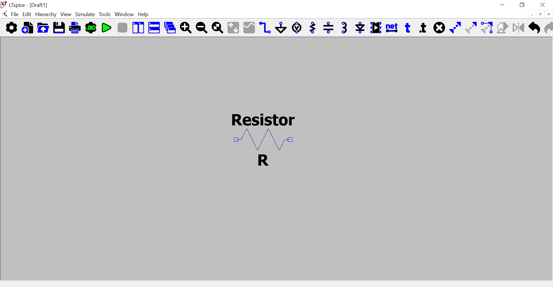
Figure 1: Key areas of the LTspice interface
Essential keyboard shortcuts
| Key | Action |
|---|---|
| P | Place a component (opens component picker) |
| W | Draw a wire between nodes |
| F4 | Place a net label (name a node) |
| G | Place a ground symbol — every circuit needs at least one |
| Ctrl+R | Rotate a component before placing |
| Escape | Cancel current action / deselect |
| Ctrl+Z | Undo |
| Space | Pan the schematic view |
| Ctrl+Scroll | Zoom in / out |
The ground rule
Every LTspice circuit needs at least one GND symbol (press G to place). Without a ground reference the simulator has no voltage reference and will refuse to run
4. Your first circuit: voltage divider
A voltage divider is the ideal starting point: two resistors in series, measuring the voltage at the midpoint. The output is V_out = V_in × R2 / (R1 + R2). Build it first, then verify with simulation.
Building the schematic
- Press P,type
voltageand place a DC voltage source (V1). Double-click it and set the value to12. - Press P,type
res, place R1 =10kand R2 =4.7kbelow it. - Press W and wire: V1 positive → top of R1 → R1 → R2 → V1 negative.
- Press G and connect a ground to the negative terminal of V1.
- Press F4, label the midpoint node
Vout.
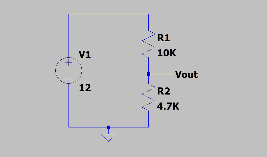
Figure 2: Voltage divider schematic in LTspice
Expected output: Vout = 12 × 4700 / 14700 ≈ 3.84 V. Verify this next with a DC operating point simulation.
5. DC operating point analysis
The DC operating point (.op) is the simplest simulation: apply all DC sources and solve for the steady-state voltage at every node; a snapshot at t=0 with capacitors open and inductors shorted.
- Go to Simulate → Edit Simulation Cmd.
- Click the DC op pnt tab and click OK. Place the
.opdirective on the canvas. - Press Run. A results window appears listing
V(Vout)at ~3.84 V.
Reading results on the schematic
After a .op run, hover the voltage probe over any wire and click to annotate its voltage directly on the schematic. Click a component to read current through it.
; KCL verification at Vout:
;   (V1 - Vout) / R1 = Vout / R2
;   (12 - Vout) / 10000 = Vout / 4700
;   → Vout = 12 × 4700 / 14700 ≈ 3.837 V  ✓
6. Transient analysis
Transient analysis simulates the circuit over a time window and captures every node voltage as a waveform — a virtual oscilloscope with unlimited probe points.
| Source type | SPICE syntax | Use case |
|---|---|---|
| SINE | SINE(0 1 1000) | 1 V peak, 1 kHz sine, 0 V offset |
| PULSE | PULSE(0 5 0 1n 1n 500u 1m) | 0→5 V pulse, 1 ns edges, 500 µs on, 1 ms period |
| PWL | PWL(0 0 1u 5 2u 5 3u 0) | Piecewise linear — arbitrary waveform |
Setting up .tran
Go to Simulate → Edit Simulation Cmd → Transient. For a 1 kHz signal, 3 ms gives a clean three-cycle view. Click OK and place the .tran 3m directive on your schematic.
Step size
LTspice chooses the internal timestep automatically. If a simulation runs unusually slowly, adding a maximum step (.tran 3m 0 1u) limits it to 1 µs.
7. Example: RC low-pass filter
An RC low-pass filter passes low frequencies and attenuates high ones. Cutoff frequency: f_c = 1 / (2π × R × C). With R = 1 kΩ and C = 100 nF, that's ~1.6 kHz.
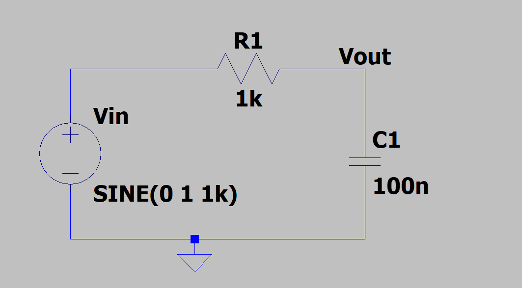
Figure 3: RC low-pass filter
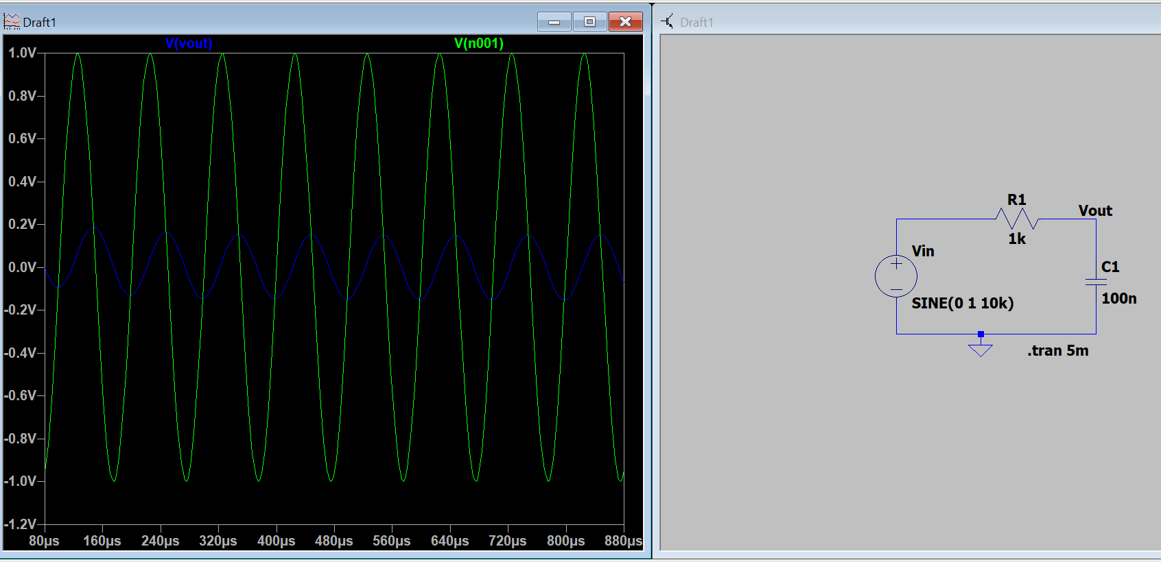
Add .tran 5m and probe both Vin and Vout. At 1 kHz the output is nearly full amplitude with a small phase lag. At 10 kHz the output is dramatically attenuated(blue waveform below)
Simulation lets you hear the circuit before you build it. Change one component value and re-run in seconds. On the bench, that's an hour of resoldering ~some wise man
8. AC analysis: frequency response
AC analysis sweeps across a frequency range and plots gain and phase — the classic Bode plot. This is how you characterise filters, amplifiers, and anything with frequency-dependent behaviour.
Setting up .ac
.ac dec 100 1 1MegThis sweeps logarithmically (decades), 100 points per decade, from 1 Hz to 1 MHz.
Set your source amplitude to AC
Double-click V1, click "Advanced," set the AC Amplitude field to 1. The DC and transient values are ignored for .ac. Forgetting this gives 0 V everywhere on the Bode plot.
After running: right-click the plot → "Add Trace" → type Vdb(Vout) for gain in decibels. You'll see the −3 dB point at 1.6 kHz, then a −20 dB/decade rolloff — exactly what theory predicts for a first-order RC filter.
Reading the Bode plot
| Measurement | How to read in LTspice |
|---|---|
| −3 dB point | Find where gain drops to −3 dB on the Vdb(Vout) trace. Press S, click the trace to place a cursor. |
| Phase margin | Add trace ph(V(Vout)) — right-click → "Add Second Y-Axis." |
| Gain at a frequency | Place cursor (S key), click trace, then click the target frequency on the axis. |
| Bandwidth | Distance between the −3 dB points for bandpass filters. |
9. Example: inverting op-amp amplifier
An inverting amplifier with gain A_v = −R_f / R_in. We'll use the UniversalOpAmp2 model included with LTspice.
- Press P, search
UniversalOpAmp2. For realistic results, useLT1001or a specific part number. - Connect the non-inverting input (+) to ground. The inverting input (−) is the summing junction.
- R_in = 10 kΩ from input source to the inverting input. R_f = 47 kΩ from output back to the inverting input.
- Connect power pins: V+ to +15 V, V− to −15 V. Op-amps will not function without supply connections.
- Set the input source:
SINE(0 0.5 1000)— 0.5 V peak, 1 kHz. - Label nodes
VinandVout.
Expected gain
R_in = 10 kΩ, R_f = 47 kΩ → gain = −4.7. A 0.5 V peak input gives ~2.35 V peak output, inverted 180°. Run .tran 3m and probe both nodes to verify.
Experiments to build intuition
| Experiment | What to do | What you'll see |
|---|---|---|
| Output clipping | Increase input to 5 V peak, rerun | Output clips at ±13–14 V. The formula stops applying. |
| Gain-bandwidth | Switch to LT1001, run .ac | Real op-amps have finite GBW. Gain × bandwidth = constant. |
| Slew rate limiting | Input = 10 kHz, 2 V peak | Output looks triangular — the op-amp can't slew fast enough. |
| Noise | Add .noise V(Vout) V1 dec 100 1 100k | Input-referred noise density vs frequency. |
10. SPICE directives cheat sheet
SPICE directives are text commands placed on the schematic (press S or Edit → SPICE Directive).
; DC Operating Point
.op

; Transient
.tran 10m              ; 10 ms, auto timestep
.tran 10m 0 1u         ; 10 ms, max step = 1 µs

; AC Sweep
.ac dec 100 1 1Meg     ; 100 pts/decade, 1 Hz–1 MHz
.ac lin 1000 100 10k   ; 1000 linear pts, 100 Hz–10 kHz

; DC Sweep
.dc V1 0 12 0.1        ; sweep V1 from 0 V to 12 V

; Parameters
.param Rf=47k Rin=10k  ; reference as {Rf} and {Rin}

; Step — run with multiple values
.step param Rf list 10k 47k 100k

; Initial Conditions
.ic V(Vout)=0

; Measure
.meas tran Vpeak MAX V(Vout)
.step is a superpower
Combine .step with a parameter to sweep component values automatically. Stepping the capacitor in an RC filter over a decade produces a family of Bode plots on a single graph.
11. Tips and good practice
Common mistakes
| Mistake | Symptom | Fix |
|---|---|---|
| No ground symbol | "No DC path to ground" — simulation aborts | Press G, connect GND to every isolated circuit island |
| Floating node | Slow convergence or wild voltages | Every node needs a DC path to ground. A 1 GΩ bleed resistor works. |
| AC amplitude not set | .ac shows 0 V everywhere | Double-click source → Advanced → AC Amplitude = 1 |
| Wrong .tran stop time | Only partial cycles visible | Stop time ≥ 3–5× the period of the lowest-frequency signal |
| Op-amp power pins unwired | Output stuck at 0 V | Connect all supply pins (V+, V−, V_EE, etc.) |
Good simulation habits
- Verify back-of-envelope first. Calculate the expected result before running. If simulation disagrees by more than a few percent, hunt for a wiring error.
- Name your nodes. Use F4 to label key nodes. "V(Vout)" in results is far clearer than "V(n001)."
- Save both .asc and .raw files. Waveform data lives in the .raw file. Share both when asking for help online.
- Comment your schematics. Use Edit → Text (T) to add notes on purpose, key frequencies, and expected values.
- Use .step for exploration. Sweep a component range automatically rather than re-running manually.
Going further
Once you're comfortable with passives and op-amps, LTspice handles BJT and MOSFET circuits, switching power supplies and RF topologies. The Analog Devices LTspice page includes hundreds of example schematics ; opening and probing real designs is one of the most effective ways to build depth.